

A calibration curve relates a known analyte concentration to an instrument response. Its slope describes the change in response per unit concentration; its intercept is the predicted response at zero concentration. A high correlation coefficient or R² alone does not demonstrate that the curve is suitable for quantitative analysis.
Use residuals, back-calculated standards and independent quality-control samples together. Acceptance criteria must come from your method, validation and approved laboratory procedures, rather than a universal R² threshold.
What does y = ax + b mean?
For a straight-line calibration, y = ax + b.
↔ 表が見切れている場合は、左右にスクロールしてご覧ください。↔ Scroll the table horizontally to see any hidden columns.
| Symbol | Meaning | Check before calculating |
|---|---|---|
| x | Analyte concentration in the measured solution | Concentration units and any dilution correction |
| y | Instrument response | Counts, peak area or an internal-standard response ratio |
| a | Slope | Response units divided by concentration units |
| b | Intercept | Response units; possible effects of background and blanks |
Calculate an unknown concentration using x = (y − b) / a. This gives the concentration in the measured solution. Conversion to the original sample may additionally require dilution, final solution volume and sample mass.
Worked example: fit a calibration and calculate a concentration
The following data are invented for teaching. They do not prescribe a required number or spacing of calibration standards.
↔ 表が見切れている場合は、左右にスクロールしてご覧ください。↔ Scroll the table horizontally to see any hidden columns.
| Standard concentration x (µg/L) | Response y (arbitrary units) |
|---|---|
| 0 | 22 |
| 1 | 118 |
| 2 | 225 |
| 3 | 316 |
| 4 | 419 |
Step 1: calculate slope and intercept
For unweighted ordinary least squares with an intercept:
a = Σ[(x − x̄)(y − ȳ)] / Σ[(x − x̄)²]
b = ȳ − a × x̄
Here x̄ = 2 and ȳ = 220. The numerator is 992 and the denominator is 10, giving a = 99.2 and b = 21.6. The fitted equation is y = 99.2x + 21.6. Use all included calibration points, rather than selecting two convenient points to draw a line.
Least squares minimizes the sum of squared response residuals. It is sensitive to outliers and should not be extrapolated casually. NIST: Linear least squares regression
Step 2: check R² and individual standards
For ordinary least squares with an intercept, R² = 1 − Σ(y − ŷ)² / Σ(y − ȳ)², where ŷ is the fitted response. In this example, the residual sum of squares is 43.6 and the total sum of squares is 98,450, so R² ≈ 0.99956.
Yet the 1 µg/L standard back-calculates to (118 − 21.6) / 99.2 ≈ 0.972 µg/L, a relative error of about −2.8%. A high R² does not mean that every concentration error is tiny. Whether these data are acceptable depends on the intended use and method-specific criteria.
Step 3: calculate the unknown
For a sample response of 270, x = (270 − 21.6) / 99.2 ≈ 2.50 µg/L. Apply additional sample-preparation factors only when they have not already been applied by the instrument software. Avoid correcting for the same dilution twice.
Slope: a sensitivity indicator, not a quality score
For y = 100x + 20, with x in µg/L and y in counts, the slope is 100 counts/(µg/L). Increasing concentration from 2 to 5 µg/L changes the predicted response by 100 × (5 − 2) = 300 counts.
A larger slope means a larger response change under the same measurement conditions. It does not automatically mean a better detection limit: noise and blank variability also matter. Compare slopes only when response definitions, units, internal-standard corrections and measurement conditions are comparable.
Instrument condition, sample introduction, integration time and matrix differences can all change slope. Compare with historical performance, internal-standard response and QC results before deciding what the change means.
Intercept: why low concentrations need extra care
The intercept is the fitted response at zero concentration. It can reflect background, blank contamination, carryover, low-level variability and correction procedures. It is not automatically identical to the measured blank.
Using the illustrative equation y = 100x + 20:
↔ 表が見切れている場合は、左右にスクロールしてご覧ください。↔ Scroll the table horizontally to see any hidden columns.
| Sample response | With intercept: (y − 20)/100 | Ignoring intercept: y/100 | Relative difference |
|---|---|---|---|
| 120 | 1.00 µg/L | 1.20 µg/L | +20% |
| 1020 | 10.00 µg/L | 10.20 µg/L | +2% |
Both differences are 0.20 µg/L, but the relative effect is much greater at low concentration. This comparison keeps the slope fixed. Refitting a line through the origin can also change the slope.
Do not force an intercept to zero simply because it looks inconvenient. A zero-intercept model requires scientific and method-validation justification. A negative intercept alone is not proof of a failed calibration either.
Correlation coefficient r versus R²
r describes the direction and strength of a linear association. R² describes the fraction of response variation explained by the fitted model. In unweighted simple linear regression with an intercept, R² = r². For weighted or zero-intercept fits, check how the software defines the reported statistic.
An R² of 0.999 does not mean that concentration errors are below 0.1%. A wide concentration range can produce a high R² while hiding substantial relative errors at the low end. Even a curved response may look highly correlated over a selected range.
ICH Q2(R2) discusses slope, intercept, correlation or determination coefficients and evaluation of deviations from the regression line. ICH Q2(R2): Validation of Analytical Procedures
Residuals reveal patterns that R² can hide
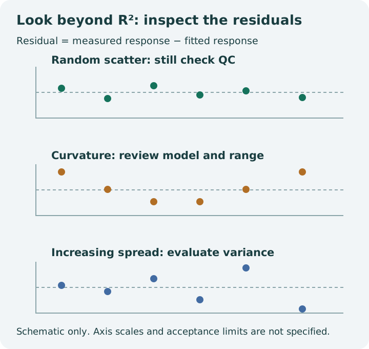
Residual = measured response − fitted response. Plot concentration on the horizontal axis and residual on the vertical axis. Examine both the size and the pattern of deviations.
↔ 表が見切れている場合は、左右にスクロールしてご覧ください。↔ Scroll the table horizontally to see any hidden columns.
| Residual pattern | Possible issue | Follow-up |
|---|---|---|
| Approximately random around zero | No obvious systematic pattern | Still assess back-calculated standards and QC |
| U-shaped or inverted U-shaped | Curvature | Investigate range, saturation or a justified alternative model |
| Increasing spread with concentration | Unequal variance | Evaluate replicate data and justified weighting |
| One large deviation | Preparation, measurement or entry problem | Investigate records and reprepare or remeasure as appropriate |
| Several consecutive residuals with the same sign | Systematic mismatch | Check model, standards, background and drift |
Do not remove a point just to improve R². Investigate the cause and follow predefined exclusion procedures. NIST: Assessing model fit
Calibration range, extrapolation and weighting
Define the range by the accuracy and precision needed for the intended measurement, not merely by the range over which the instrument returns a signal.
At the lower end, blanks, noise and intercept effects become relatively important. Including a low standard in a fit does not by itself establish a validated limit of quantification. At the upper end, saturation and other nonlinear effects may require dilution, a reduced range or different conditions.
Avoid reporting an extrapolated result simply because the software can calculate it. If the response exceeds the upper standard, dilute and remeasure within the validated range when appropriate. Results below the lowest standard also require the method's reporting rules.
Unweighted least squares minimizes squared response residuals. When response variance increases with concentration, higher-concentration points can strongly influence the fit. Weighting such as 1/x or 1/x² may be considered when justified by the error structure. Handle the zero-concentration point explicitly: those expressions are undefined at x = 0. Select weighting using residuals, back-calculated standards, independent QC and validation, rather than R² alone.
A practical calibration review checklist
- Confirm standard concentrations, units and preparation records.
- Check that the validated range covers the intended samples and QC levels.
- Compare slope and intercept with expected performance and blanks.
- Distinguish r from R² and verify the regression model and weighting.
- Examine residual patterns and back-calculated standard concentrations.
- Review independent QC, spike recovery and internal-standard response as applicable.
- Dilute or remeasure out-of-range samples according to the method.
- Record the reasons for any excluded standards and corrective action.
Frequently asked questions
Is a correlation coefficient above 0.999 sufficient?
No universal threshold establishes fitness for purpose. Follow the applicable method and also examine residuals, back-calculated standards and QC. High correlation can coexist with unacceptable low-level errors.
Does a lower R² mean that measurement must stop immediately?
Follow the approved acceptance criteria first. Then investigate standards, measurement sequence, residuals, blanks and independent QC. Do not retrospectively remove points or change the range merely to recover a preferred R².
Can a steeper slope alone establish a lower detection limit?
No. Response variability and blanks also matter. A detection or quantification limit calculated from a formula still needs an appropriate performance assessment.
Can I compare calibrations from different days?
Yes, when units, response definitions and conditions are comparable, as part of an established control procedure. Interpret changes alongside QC and instrument-performance information.
From calibration to a reportable result
Evaluate slope, intercept, residuals, standard back-calculations, QC and the concentration range together. A favorable R² is useful supporting information, not a substitute for demonstrating that the method meets its intended purpose.
For the broader calibration framework, see IUPAC: Guidelines for calibration in analytical chemistry and Eurachem: Method validation guides.
This guide addresses general straight-line calibration. Regulatory methods may specify particular standard levels, regression models, weighting and QC rules. Use the applicable standard, validated method and approved SOP for actual acceptance decisions.
Reproduce the example in Excel
Place concentration values 0, 1, 2, 3, 4 in A2:A6 and responses 22, 118, 225, 316, 419 in B2:B6. Use row 1 for column headings.
↔ 表が見切れている場合は、左右にスクロールしてご覧ください。↔ Scroll the table horizontally to see any hidden columns.
| Result | Cell | Formula or input | Expected value |
|---|---|---|---|
| Slope | E2 | =SLOPE(B2:B6,A2:A6) | 99.2 |
| Intercept | E3 | =INTERCEPT(B2:B6,A2:A6) | 21.6 |
| R² | E4 | =RSQ(B2:B6,A2:A6) | Approximately 0.99956 |
| Sample response | E6 | Enter 270 | 270 |
| Concentration (µg/L) | E7 | =(E6-E3)/E2 | Approximately 2.50 |
Specify response values first, concentration values second. Use an XY scatter chart. These formulas describe unweighted linear regression with a fitted intercept; do not use them unchanged for weighted or zero-intercept fits. Check residuals, back-calculated standards and independent quality-control samples. Apply dilution and original-sample conversion separately.